Audio Classification using FastAI and On-the-Fly Frequency Transforms
Originally published on Medium / Towards Data Science on November 28, 2018. Reposted here for archival purposes. Code is available at github.com/jhartquist/fastai_audio.
Introduction
While deep learning models are able to help tackle many different types of problems, image classification is the most prevalent example for courses and frameworks, often acting as the "hello, world" introduction. FastAI is a high-level library built on top of PyTorch that makes it extremely easy to get started classifying images, with an example showing how train an accurate model in only four lines of code. With the new v1 release of the library, an API called data_block allows users a flexible way to simplify the data loading process. After competing in the Freesound General-Purpose Audio Tagging Kaggle competition over the summer, I decided to repurpose some of my code to take advantage of fastai's benefits for audio classification as well. This article will give a quick introduction to working with audio files in Python, give some background around creating spectrogram images, and then show how to leverage pretrained image models without actually having to generate images beforehand.
All the code used to generate the content of this post will be available in this repository, complete with example notebooks.
Audio Files to Images
At first, it may seem a little strange to classify audio files as images. Images are 2-dimensional after all (with a possible 3rd dimension for RGBA channels), and audio files have a single time dimension (with a possible 2nd dimension for channels, for example stereo vs mono). In this post, we'll only be looking at audio files with a single channel. Every audio file also has an associated sample rate, which is the number of samples per second of audio. If a 3 second audio clip has a sample rate of 44,100 Hz, that means it is made up of 3*44,100 = 132,300 consecutive numbers representing changes in air pressure. One of the best libraries for manipulating audio in Python is called librosa.
clip, sample_rate = librosa.load(filename, sr=None)
clip = clip[:132300] # first three seconds of file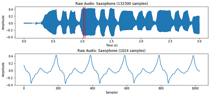
While this representation does give us a sense of how loud or quiet a clip is at any point in time, it gives us very little information about which frequencies are present. A very common solution to this problem is to take small overlapping chunks of the signal, and run them through a Fast Fourier Transform (FFT) to convert them from the time domain to the frequency domain. After running each section through an FFT, we can convert the result to polar coordinates, giving us magnitudes and phases of different frequencies. While the phases information can be useful in some contexts, we mostly use the magnitudes, and convert them to decibel units because our ears percieve sound on a logarithmic scale.
n_fft = 1024  # frame length
start = 45000 # start at a part of the sound thats not silence
x = clip[start:start+n_fft]
X = fft(x, n_fft)
X_magnitude, X_phase = librosa.magphase(X)
X_magnitude_db = librosa.amplitude_to_db(X_magnitude)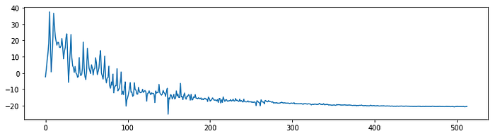
Taking an FFT of size 1024 will result in a frequency spectrum with 1024 frequency bins. The second half of the spectrum is redundant however, so in practice we only use the first (N/2)+1 bins, which is 513 in this case.
To generate information about the whole file, we can take an FFT of a 1024 sample window, and slide it by 512 samples (hop length) so that the windows overlap with each other. For this three second file, that will give us 259 frequency spectrums, which we can then view as a 2-dimensional image. This is called a short-time Fourier Transform (STFT), and it allows us to see how different frequencies change over time.
stft = librosa.stft(clip, n_fft=n_fft, hop_length=hop_length)
stft_magnitude, stft_phase = librosa.magphase(stft)
stft_magnitude_db = librosa.amplitude_to_db(stft_magnitude)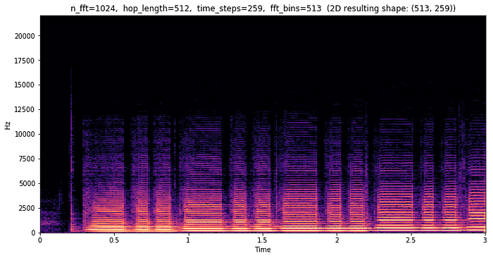
In this example, we can see that almost all of the interesting frequency data is below 12,500 Hz. In addition to there being a lot of wasted bins, this does not accurately display how humans perceive frequencies. Along with loudness, we also hear frequencies on a logarithmic scale. We would hear the same "distance" of frequencies from 50 Hz to 100 Hz as we would between 400 Hz and 800 Hz.
These are some of the reasons why many people use melspectrograms which transform the frequency bins into the mel scale. Librosa allows us to easily convert a regular spectrogram into a melspectrogram, and lets us define how many "bins" we want to have. We can also specify a minimum and maximum frequency that we want our bins to be divided into.
mel_spec = librosa.feature.melspectrogram(
    clip,
    n_fft=n_fft,
    hop_length=hop_length,
    n_mels=n_mels,
    sr=sample_rate,
    power=1.0,
    fmin=fmin,
    fmax=fmax,
)
mel_spec_db = librosa.amplitude_to_db(mel_spec, ref=np.max)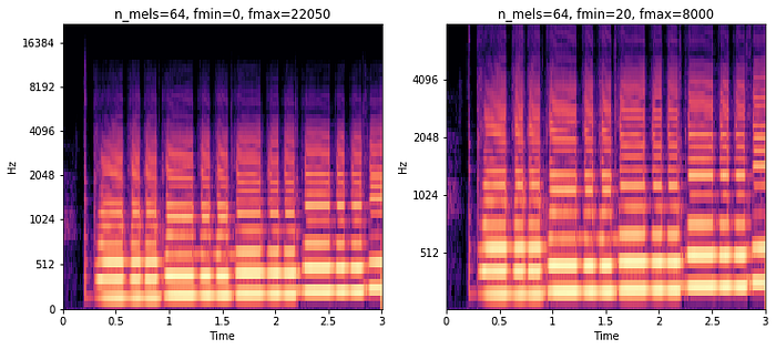
In each of these melspectrograms, I used 64 frequency bins (n_mels). The only difference is that on the right, I specified that I only care about frequencies between 20Hz and 8000Hz. This greatly reduces the size of each transform from the original 513 bins per time step.
Classifying Audio Spectrograms with fastai
While it is possible to classify raw audio waveform data, it is very popular to use image classifiers to classify melspectrograms, and it works pretty well. In order to do this we have to convert our whole dataset to image files using similar code as above. This took me about 10 minutes of processing time using all the CPUs on my GCP instance. I used the following parameters for generating the melspectrogram images:
n_fft = 1024
hop_length = 256
n_mels = 40
f_min = 20
f_max = 8000
sample_rate = 16000
For the rest of this post, I've used the NSynth Dataset by the Magenta team at Google. It is an interesting dataset composed of 305,979 musical notes, each 4 seconds long. I trimmed the dataset down to only the acoustically generated notes to make things a little more manageable. The goal was to classify which instrument family each note was generated with out of 10 possible instrument families.
Using fastai's new data_block API, it becomes very easy to build a DataBunch object with all the spectrogram image data along with their labels — in this example I grabbed all of the labels using a regex over the filenames.
NSYNTH_IMAGES = 'data/nsynth_acoustic_images'
instrument_family_pattern = r'(\w+)_\w+_\d+-\d+-\d+.png$'
data = (ImageItemList.from_folder(NSYNTH_IMAGES)
          .split_by_folder()
          .label_from_re(instrument_family_pattern)
          .databunch())
Once I had my data loaded, I instantiated a pretrained Convolutional Neural Network (CNN) called resnet18, and fine-tuned it on the spectrograms.
learn = create_cnn(data, models.resnet18, metrics=accuracy)
learn.fit_one_cycle(3)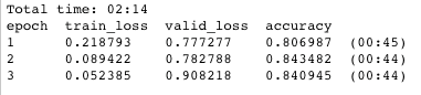
In only 2 minutes and 14 seconds I was left with a model that scored 84% accuracy on the validation set (a completely separate set of instruments from the training set). While this model is definitely overfitting, this is without data augmentation or regularization of any kind, a pretty good start!
By utilizing fastai's ClassificationInterpretation class, we can take a look at where the mistakes are coming from.
interp = ClassificationInterpretation.from_learner(learn)
interp.plot_confusion_matrix(figsize=(10, 10), dpi=60)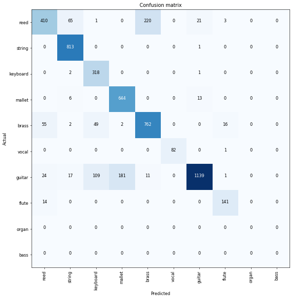
It looks like mallets are getting confused with guitars, and reeds are being confused with brass instruments the most. Using this information, we could look more closely at the spectrograms of those instruments, and try to decide if there are better parameters we could use to differentiate between them.
Generating Spectrograms During Training, why?
If classifying audio from images works so well, you might ask why it would be beneficial to generate spectrograms during training (as opposed to before). There are a few good reasons for this:
- Time to generate images. In the previous example, it took me over 10 minutes to generate all the spectrogram images. Every time I want to try out a different set of parameters, or maybe generate a plain STFT instead of melspectrogram, I'd have to regenerate all those images. This makes it hard to test a lot of different configurations quickly.
- Disk space. Similarly, every time I generate a new set of images, they can take up large amounts of hard-drive space depending on the size of the transforms and the dataset itself. In this case, my generated images took up over 1GB of storage.
- Data augmentation. One of the most effective strategies for improving performance with image classifiers is to use data augmentation. The regular image transforms however, (rotating, flipping, cropping, etc) do not make as much sense for spectrograms. It would be better to transform audio files in the time domain, and then convert them to spectrograms right before sending them to a classifier.
- GPU vs CPU. In the past, I always did the frequency transforms using librosa on CPU, but it would be nice to utilize PyTorch's
stftmethod on the GPU since it should be much faster, and be able to process batches at a time (as opposed to 1 image at a time).
Generating Spectrograms During Training, how?
Over the past few days I've been experimenting with an idea to create a new fastai module for audio files. After reading the great new fastai documentation, I was able to write some basic classes to load raw audio files and generate the spectrograms as batches on the GPU using PyTorch. I also wrote a custom create_cnn function that would take pretrained image classifiers, and modify them to work on a single channel (spectrogram) instead of the 3 channels they were originally trained for. To my surprise, the code runs almost as fast as the image classification equivalent, with no extra step of generating actual images. Setting up my data now looks like this:
tfms = get_frequency_batch_transforms(n_fft=n_fft,
                                      n_hop=n_hop,
                                      n_mels=n_mels,
                                      sample_rate=sample_rate)
data = (AudioItemList
            .from_folder(NSYNTH_AUDIO)
            .split_by_folder()
            .label_from_re(instrument_family_pattern)
            .databunch(bs=batch_size, tfms=tfms))
The fastai library supports a nice way to preview batches as well:
data.show_batch(3)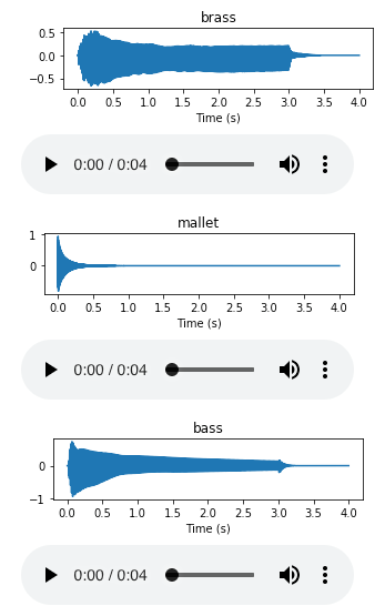
Fine-tuning on a pretrained model is exactly the same as before, only this time the first convolutional layer is being modified to accept a single input channel (thanks to David Gutman on the fastai forums).
learn = create_cnn(data, models.resnet18, metrics=accuracy)
learn.fit_one_cycle(3)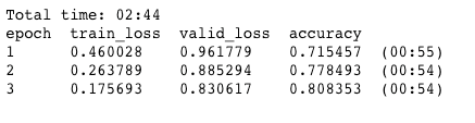
This time the training takes only 30 seconds longer, and has only slightly lower accuracy after 3 epochs with 80% on the validation set! Generating images on the CPU before took over 10 minutes when doing it one at time. This opens up the possibility for much more rapid experimentation with tuning spectrogram parameters and as well as computing spectrograms from augmented audio files.
Future Work
Now that its possible to generate different spectral representations on the fly, I'm very interested in trying to get data augmentation working for raw audio files. From pitch shifting, to time stretching (methods available in librosa), to simply taking random segments of audio clips, there is a lot to experiment with.
I am also interested in how much better the results would be the pretrained models used here had actually been trained on audio files and not image files.
Thanks for taking the time to read my first blog post! Please let me know if you have any corrections or comments. Once again, you can view all the code and full notebooks over at github.com/jhartquist/fastai_audio.
Resources
- FastAI docs
- PyTorch v1.0 docs
- torchaudio: Heavy inspiration for this article
- Great intro to Fourier Transform: https://jackschaedler.github.io/circles-sines-signals/dft_introduction.html
- Speech Processing for Machine Learning: Filter banks, Mel-Frequency Cepstral Coefficients (MFCCs) and What's In Between
- Highly recommended course on audio signal processing in Python: Audio Signal Processing for Musical Applications